Selección de Variables (Shinkage Methods)

Mariano Rivera

Ver $\S$3.4 in [1]

[1] T. Hastie, R. Tibshirani and J Friedman, The elements of Statistical Learning, 2nd Ed. Springer, 2009.

import numpy as np 
import sklearn as skl
import matplotlib.pyplot as plt
from PIL import Image

Regresión Ridge

El propósito es mantener el menor número de perdictores descartando el resto. Con ello se gana interpretabilidad y mejora el error de generalización

Asumamos una muestra aleatoria $x$ de tamaño m:

(1)
$\mathbf{X} = \begin{bmatrix} x_1^\top, \\ x_2^\top, \\ \vdots \\ x_m^\top \end{bmatrix}$

con $x_i \in \mathbb{R}^n$.

Donde denotamos $x_i$ la $i$-ésima observación. Luego $X$ denota la variable de entrada genérica, $X_j$ su $j$-ésimo componente; como $x_{ij}$ el $j$-ésimo componente de la $i$-ésima observación.

En estas notas usemos la regresión lineal como ilustración:

(2)
$y_i = b + x_i ^\top \theta + \eta_i$

donde $\theta \in \mathbb{R}^{n}$, $b \in \mathbb{R}^1$ el interceptor.

Luego la regresion Ridge esta dada por:

(3)
$b^{ridge},\theta^{ridge} = \underset{b,\theta}{\arg\min} \, \| y - b - \mathbf{X} \theta_{1\ldots n} \|^2 + \lambda \| \theta \|_2^2$

con el parámetro de complejidad $\lambda \ge 0$ que controla el grado de encogimiento.

Forma centrada de Ridge

Note que la penalización no se hace sobre el interceptor $b$.

De hecho es fácil notar que si se usan datos centrados:
$x_{ij} \leftarrow x_{ij}-\bar x_j$
Entonces en toma una forma mas simple, el iterceptor estará dado por

(4)
$b^{ridge} \equiv \bar y = \frac{1}{m} \sum_i y_j$

luego hacemos:

$y_{i} \leftarrow y_{i}-\bar y$

Lo que nos lleva a la forma centrada Ridge:

(5)
$\theta^{ridge} = \underset{\theta}{\arg\min} \, \| y - \mathbf{X}\theta \|^2 + \lambda \| \theta \|^2$

Consideremos la versión simplificada (centrada) en (5), luego resolviendo para el gradiente:

$\theta^{ridge} = (\mathbf{X^\top X + \lambda\,I})^{-1} \mathbf{X^\top} \mathbf{Y}$

Es decir, le esta sumando $\lambda$ a la diagonal de la matriz Hessiana $\mathbf{X^\top X}$, lo que ayuda a mejorar su condición

Forma de Mínimos cuadrados de Ridge

Proposición.

La Regularización Lineal Ridge (5) es equivalente al problema de mínimos cuadrados:

(6)
$\theta^{ridge} = \underset{\theta}{\arg\min} \, \| b - \mathbf{A}_\lambda \theta \|_2^2$

Donde

$\mathbf{A}_\lambda \overset {def}{=} \begin{bmatrix} \mathbf{X} \\ \sqrt{\lambda} \mathbf{I} \end{bmatrix},$

$b \overset {def}{=} \begin{bmatrix} y \\ 0 \end{bmatrix}$

Proof.

Es fácil demostrar que

$\| y - \mathbf{X}\theta \|_2^2 + \lambda \| \theta \|_2^2 = \| b -\mathbf{A}_\lambda\theta \|_2^2$

Aquí esta el álgebra
$\| y - \mathbf{X}\theta \|^2 + \lambda \| \theta \|^2 = (y - \mathbf{X}\theta)^\top (y - \mathbf{X}\theta) + \lambda \theta^\top \theta \\ \;\;\;\;\;\;\;\;\;\;\;\;\;\;\;\;\;\;\;\;\;\;\;\;\;\;\;\; = \begin{bmatrix} y -\mathbf{X}\theta \\ 0- \sqrt{\lambda} \mathbf{I} \theta \end{bmatrix}^\top \begin{bmatrix} y -\mathbf{X}\theta \\ 0- \sqrt{\lambda} \mathbf{I} \theta \end{bmatrix} \\ \;\;\;\;\;\;\;\;\;\;\;\;\;\;\;\;\;\;\;\;\; = \begin{bmatrix} b - \mathbf{A}_\lambda \theta \end{bmatrix}^\top \begin{bmatrix} b -\mathbf{A}_\lambda \theta \end{bmatrix} \\ \;\;\;\;\;\;\;\; = \| b -\mathbf{A}_\lambda\theta \|_2^2.$

Forma restringida de Ridge

El potencial (3) puede escrito en forma equivalente como un problema con restricciones:

(7)
$b^{ridge}, \theta^{ridge} = \underset{b,\theta}{\arg\min} \, \| y - b - \mathbf{X} \theta \|^2 \;\;\;\;\; \text{sujeto a } \;\;\; \| \theta \|^2 \le t$

para algun valor de $t$ en correspondencia a $\lambda$. El programa (7) explícitamente impone una restricción en el tamaño de los parámetros.

Dado que se penaliza el cuadrado del la magnitud, el inconveniente principal de la regresión Ridge es que se promoverá que aparezcan varios valores pequeños en vez de uno grande (no promueve ralez).

# Modelo Cuadrático: y = x'Ax+ x'b = x'(Ax+b)

# matriz de rotacion (eigen vectores)
alpha=np.pi/12
R = np.matrix([[np.cos(alpha),np.sin(alpha)],[-np.sin(alpha),np.cos(alpha)]]) 
# eigenvalores
D = np.matrix([[1,0],[0,0.2]]) 
# Hessiano
A = 3*np.dot(R,np.dot(D,R.T))
# translacion
b = np.matrix([[-1],[-2]])

#Region a "plotear"
delta = 0.05
x1 = np.arange(-0.5, 2.0, delta)
x2 = np.arange(-0.5, 2.0, delta)
X1, X2 = np.meshgrid(x1, x2)

# calculo del modelo cuadratico
rows, cols = X1.shape
Y = np.zeros((rows,cols))
for i in range(rows):
    for j in range(cols):
        x = np.matrix([X1[i,j],X2[i,j]]).T
        Y[i,j]=  np.dot(x.T, np.dot(A,x) + b)

Para la norma $L_p$:

$L_p(x) \overset{def}{=} \left[ \sum_i |x_i|^p \right]^{\frac{1}{p}}$

y toma valores interesantes para $0<p\le 1$.

Por ejemplo, para el caso ilustrado en dos dimensiones:

$L_{p}([x,y]^T) = \left[ x^p + y^p \right]^{\frac{1}{p}} =1$

luego

$y = \left[1-x^{p}\right]^{\frac{1}{p}}$

plt.figure(figsize=(8,8))

# El potencial Quadrático
levels = np.arange(-2.0, 9, 0.2)
CS = plt.contour(X1, X2, Y, levels,
                 linewidths=1,
                 extent=(-3, 3, -2, 2))

#CS = plt.contour(X1, X2, Y)
plt.clabel(CS, inline=1, fontsize=10)
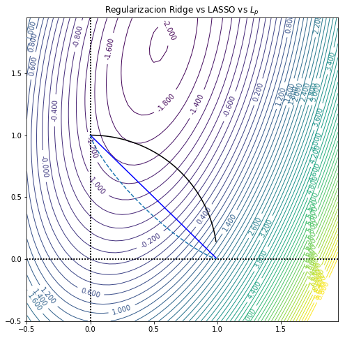
plt.title('Regularizacion Ridge vs LASSO vs $L_p$ ')
#-------------------------------------
#Penalizacion L_2
x = np.arange(0,1,0.01)
y = np.sqrt(1-np.power(x,2))
plt.axvline(0.0,ls='dotted', color='k')
plt.axhline(0.0,ls='dotted', color='k')
plt.plot(x,y,'k')
#-------------------------------------
#Penalizacion L_1
x = np.arange(0,1,0.01)
y = 1-x
plt.axvline(0.0,ls='dotted', color='k')
plt.axhline(0.0,ls='dotted', color='k')
plt.plot(x,y,'b')
#-------------------------------------
#Penalizacion L_p, con p=0.4
x = np.arange(0,1,0.01)
p = .8
y = np.power(1-np.power(x,p),1/p)
plt.axvline(0.0,ls='dotted', color='k')
plt.axhline(0.0,ls='dotted', color='k')
plt.plot(x,y,'--')
#-------------------------------------

plt.show()

Notemos que conforme $p\downarrow 0$, el punto en que la fontera (lineas mostradas) de la región factible y las curvas de nivel de la función objetivo son tangentes se acerca al eje, lo que resulta en una solución mas informativa (que tienen menor entropía o se aaproxima más aser una variable indicadora).

Equivalencia en Minimización L1 y Programación Lineal

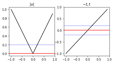
En una dimensión es fácil observar la equivalencia entre el problema de optimización de valor absoluto

$\min_x |x|$

y el LP

$\min_\theta \,\theta\\ \text{s.a.} -\theta \le x \le \theta \\ \theta \ge 0$

Esto se puede generalizar a $n$ dimensiones como el problema de optimización $L_1$

$\min_x \, \| Ax-b \|_1$
Con su equivalente LP

$\min_{\theta \in \mathbb{R}^n} \,\mathbf{1}^\top\theta\\ \text{s.a.} \; -\theta \preceq Ax-b \preceq \theta \\ \theta \succeq 0$

plt.figure(figsize=(6,3))
#-------------------------------------
plt.subplot(121)
plt.title('$|x|$')
x = np.arange(-1,1,0.1)
y = np.abs(x)
plt.plot(x,y,'k')
plt.axhline( 0.2,ls='dotted', color='b')
plt.axhline(0.0, color='r')
#-------------------------------------
plt.subplot(122)
plt.title('$-t, t$')
x = np.arange(-1,1,0.1)
y = np.abs(x)
plt.plot(x,x,'k')
plt.axhline( 0.2,ls='dotted', color='b')
plt.axhline(-0.2,ls='dotted', color='b')
plt.axhline(0.0, color='r')
#-------------------------------------
plt.show()

Regresión LASSO

La regresion LASSO esta dada por:

(8)
$b^{lasso}, \theta^{lasso} = \underset{b,\theta}{\arg\min}\, U_{l}(b,\theta) = \frac{1}{2}\| y - b - \mathbf{X} \theta \|^2 + \lambda \| \theta \|_1$

con el parámetro de complejidad $\lambda \ge 0$ que controla el grado de encojimiento.

Propondremos resolver este problema iterando dos pasos (a la vez el segundo paso será revisado con detalle)

Dados unos prametros $\theta$ iniciales, iterar:

1. Calcular el interceptor $b^{k+1}$ resolviendo $\partial U(b,\theta) /\partial b =0$ con $\theta$ fija:
   $b^{k+1} = \frac{1}{m}\mathbf{1}^\top (\mathbf{X}\theta^{k} -y)$
2. Actualizar
   $y \leftarrow y- b^{k+1}$
3. Resolver
   $\theta^{k+1} = \underset{b,\theta}{\arg\min}\, U_{l}(b,\theta) = \frac{1}{2}\| y - \mathbf{X} \theta \|^2 + \lambda \| \theta \|_1$

Los pasos son iterados hasta convergencia. El punto es ¿como se resuelve el paso 3?

Forma Restingida de la Regresión LASSO

Similarmente a la regresión Ridge, se puede demostrar que (9) tienen una forma equivalente con restricciones:

(10)
$\;\;\;\;\;\;\;\; \theta^{lasso} = \underset{\theta \in \mathbb{R}^n}{\arg\min} \, \| y - \mathbf{X} \theta \|^2 + \lambda t \\ \text{sujeto a } \;\;\; t - \theta \ge 0 \\ \;\;\;\;\;\;\;\;\;\;\;\; t + \theta \ge 0 \\ \;\;\;\;\;\;\;\;\;\;\;\;\;\; t \ge 0$

para algún valor de $t$ en correspondencia a $\lambda$. El programa (10) explícitamente impone una restricción en el tamaño de los parámetros.

Regresión LASSO Algoritmo Shooting

Propuesto para LASSO por W. J. Fu [2], el asesor de Tibsharini. Pero en su momento no valorado por Tibsharini.

Tibsharini & Hastie lo prueban, concluyen que falla en base a que la Implementación (equivocada) de Hastie no funciona (segun sus propias palabra en Tutoriales).

Hasta que es usado por Friedman en Elastic Net y funciona, Lo usan T-H-F en LASSO, 2006!

Ahora, Tibsharini & Hastie son unos de sus mayores difusores.

Gautam V. Pendse, A Tutorial on LASSO an the “shooting algorithm”,
[online] http://gautampendse.com/software/lasso/webpage/lasso_shooting.html

Ver también algoritmo LARS.

[2] W. J. Fu. Penalized Regressions: The Bridge Versus the Lasso. Journal of Computational and Graphical Statistics, 7:397-416, 1998.

Análisis en Mínimos cuadrados 1D

Primero haremos una reflexion para el caso del problema de mínimos cuadrados unidimensional:

(11)
$\underset{\theta \in \mathbb{R}^1}{\arg\min} \frac{1}{2} \| y_i - x_i \theta \|^2$

que tiene como solución:

$\theta^* = \frac{x_i^\top y_i}{x_i^\top x_i}$

asumiendo $x_i, y_i \ne 0$, lo cual hace que nuestro problema tenga sentido. Entonces $\theta^*= 0$ ssi $x_i^\top y_i =0$.

Bueno, los métodos que penalizan la norma incluyen a 0 en la región factible, de hecho es a donde tiende a encoger la solución. Por lo que, no importa que penalización de norma se adicione a (11), la solución seguira siendo $\theta^*= 0$.
Esto es:

La solución a
(12)
$\underset{\theta \in \mathbb{R}^1}{\arg\min} \frac{1}{2} \| y_i - x_i \theta \|^2 + \lambda \| \theta \|_V$

es $\theta^*= 0$ si $x_i^\top y_i =0$ dado que $\| 0 \|_V =0$.

Algoritmo Shooting

Consideremos el caso (12) para LASSO en caso que $x_i^\top y_i \ne 0$

(13)
$\underset{\theta \in \mathbb{R}^1}{\arg\min} \frac{1}{2} \| y_i - x_i \theta \|^2 + \lambda | \theta |$

que podemos escribir en forma restringida

(14)
$\underset{\theta \in \mathbb{R}^1}{\arg\min} \, \frac{1}{2} \| y_i - x_i \theta \|^2 + \lambda t \\ \text{sujeto a } \;\;\; t - \theta \ge 0 \\ \;\;\;\;\;\;\;\;\;\;\;\; t + \theta \ge 0 \\ \;\;\;\;\;\;\;\;\; t \ge 0$

Para resolver el problema, escribimos el Lagrangiano

(15)
$\mathcal{L} (\theta, t, \lambda, s_1, s_2, \pi) = \frac{1}{2}\| y_i - x_i \theta \|^2 + \lambda t - s_1(t-\theta) - s_2(t+\theta) - \pi \,t$

Con KKTs:

(16)
$\frac{\partial \mathcal{L}}{\partial \theta} =0 \rightarrow -x_i^\top y_i + \theta x_i^\top x_i + s_1 - s_2 \\ \;\;\;\;\;\;\;\;\; \rightarrow \;\;\; \theta x_i^\top x_i = x_i^\top y_i + s_2 - s_1$

(17)
$\frac{\partial \mathcal{L}}{\partial t} =0 \rightarrow \;\;\; \lambda = s_1+s_2 + \pi$

(18)
$s_1(t-\theta)=0$

(19)
$s_2(t+\theta)=0$

(20)
$\;\;\;\;\;\;\; \pi \, t =0$

(21)
$t,s_1, s_2,\pi \succeq 0 \;\;\;$

Caso General A. $t=0$

Entonces la solución es la trivial: $\theta =0$. Se obtiene directamente de las restricciones $-t\le \theta \le t$

Caso General B. $t>0$.

Entonces, $\pi = 0$ por (20) y de (17):

(22)
$\lambda = s_1+s_2$

Caso B.1: Asumimos $y_i^\top x_i - \lambda >0$:

de (22)

(23)
$s_1 =\lambda - s_2$

y sustitutendo en (16): $\theta x_i^\top x_i = x_i^\top y_i - \lambda +2s_2$.
Ahora, notamos que

1. Dado que $x_i\ne 0: \,\, x_i^\top x_i >0$,
2. Por la suposición del caso: $y^\top x - \lambda >0$,
3. Por (21): $s_2 \ge 0$
   Usando esto, tenemos que

(24)
$\theta \,\, \underbrace{x_i^\top x_i}_{>0} = \underbrace{x_i^\top y_i - \lambda}_{>0 \text{ por suposición}} \underbrace{+ \, 2s_1}_{\ge 0} >0$

Por lo tanto $\theta >0$. Luego de (19), como $(t+\theta) >0 \rightarrow s_2=0$, por la complementariedad estricta. Y tenemos:

(25)
$\theta = \frac {x_i^\top y_i - \lambda}{x_i^\top x_i}$

Caso B.2: Asumimos $y_i^\top x_i + \lambda <0$:

de (22):

(26)
$s_2 =\lambda - s_1$

y sustitutendo en (16): $\theta x_i^\top x_i = x_i^\top y_i + \lambda -2s_1$.
Ahora, notamos que

1. Dado que $x_i\ne 0: \,\, x_i^\top x_i <0$,
2. Por la suposición del caso: $y^\top x - \lambda >0$,
3. Por (21): $s_1 \ge 0$
   Usando esto, tenemos que

(27)
$\theta \,\, \underbrace{x_i^\top x_i}_{>0} = \underbrace{x_i^\top y_i + \lambda}_{<0 \text{ por suposición}} \underbrace{- \, 2s_1}_{\le 0} <0$

Por lo tanto $\theta <0$. Luego de (19), como $(t-\theta) >0 \rightarrow s_1=0$, por la complementariedad estricta. Y tenemos:

(28)
$\theta = \frac {x_i^\top y_i + \lambda}{x_i^\top x_i}$

Caso B.3: Asumimos $ - \lambda \le y_i^\top x_i \le \lambda $:

Ensayemos $\theta >0$,

1. luego $(t+\theta)>0$ e implica $s_2=0$.
2. y $\theta = \frac {x_i^\top y_i - \lambda}{x_i^\top x_i}$; pero como $x_i^\top y_i - \lambda <0$ entonces $\theta<0$. Lo que contradice la suposición inicial.

Entonces ensayemos $\theta <0$,

1. luego $(t-\theta)>0$ e implica $s_1=0$.
2. y $\theta = \frac {x_i^\top y_i + \lambda}{x_i^\top x_i}$; pero como $x_i^\top y_i + \lambda >0$ entonces $\theta>0$. Lo que contradice la suposición inicial.

Ya que $\theta \nless 0$ ni $\theta \ngtr 0$, la única forma de resolver la contradicción es hacer

(29)
$\theta = 0$
y los multiplicadores de Lagrange estarán dados por

(30)
$s_1 = \frac {\lambda + x_i^\top y_i}{2}$

(31)
$s_2 = \frac {\lambda - x_i^\top y_i}{2}$

Proposición. Algoritmo Shoothing 1D

Sea el problema LASSO 1D con $x_i y_i \ne 0$;

(13)
$\underset{\theta \in \mathbb{R}^1}{\arg\min} \frac{1}{2} \| y_i - x_i \theta \|^2 + \lambda | \theta |$
que podemos escribir en forma restringida

(14)
$\underset{\theta \in \mathbb{R}^1}{\arg\min} \, \frac{1}{2} \| y_i - x_i \theta \|^2 + \lambda t \\ \text{sujeto a } \;\;\; t - \theta \ge 0 \\ \;\;\;\;\;\;\;\;\;\;\;\; t + \theta \ge 0 \\ \;\;\;\;\;\;\;\;\; t \ge 0$

Entonces, la solución se calcula mediante

(32)
$\theta^* = \left\{\begin{matrix} \frac {x_i^\top y_i - \lambda}{x_i^\top x_i} & y_i^\top x_i > \lambda \\ 0 & - \lambda \le y_i^\top x_i \le \lambda \\ \frac {x_i^\top y_i + \lambda}{x_i^\top x_i}& y_i^\top x_i < - \lambda \end{matrix} \right.$

Algoritmo Soothing para LASSO

Para resolver el problema de regresión lineal LASSO centrado dado por (9)

(9)
$\theta^{*} = \underset{\theta}{\arg\min}\, h(\theta) = \frac{1}{2}\| y - \mathbf{X} \theta \|^2 + \lambda \| \theta \|_1$

se usa la estrategia siguiente:

• Inicialice $\theta = \theta_0$; por ejemplo, con la solución de mínimos cuadrados.
• For $k = 1,2,\ldots, K$

$\qquad$ - Compute $f_k = h(\theta)$

$\qquad$ - For $i = 1,2,\ldots, n$

$\qquad \qquad$ 1. Usando el valor actual para $\theta^{(-i)}$, resuelva el problema 1D c.r.a $\theta_i$ mediante (32):

(33)
$\underset{\theta \in \mathbb{R}^1}{\min} h'(\theta_i) = \frac{1}{2} \| y_i - x_i \theta \|_2^2 + \lambda | \theta_i | + \lambda \| \theta^{(-i)}\|_1$

$\qquad \qquad \quad$ donde $y_i = y - \mathbf{X}^{(-i)}\theta^{(-i)}$

$\qquad \qquad$ 2. Suponga que $\theta_i^*$ es la solución a (33), entonces actualizar el vector $\theta$: $\theta_i = \theta_i^*$ y dejando los demás elementos sin cambio.

Este algoritmo es del tipo descenso coordenado y converge al mínimo en tanto $K\rightarrow \infty$.

Red Elástica (Elastic Net)

La regresión usando la penalización Red Elástica esta dada por:

(34)
$b^{en}, \theta^{en} = \underset{b,\theta}{\arg\min}\, E_{e}(b,\theta) = \frac{1}{2}\| y - b - \mathbf{X} \theta \|^2 + \lambda_1 \| \theta \|_1 + \lambda_2 \| \theta\|_2^2$

con el parámetro $\lambda_1 > 0$ que promueve ralez y el parámetro $\lambda_2 >0$ que controla el grado de encogimiento.

Es posible introducir, el Término de Ridge en el términos de datos (prímer potencial) mediante la transformación vista de Ridge a mínimos cuadrados y usar el solucionador de LASSO.

Método de los Multiplicadores con Direcciones Alternadas para LASSO

[2] Boyd, notes on ADMM [online], Alternating Direction Multipliyig Method (ADMM) for LASSO

El problema LASSO se puede reescribir como

$\min_{x,z} \; \frac{1}{2}\| Ax - b\|^2_2 + \lambda \| z\|_1 \\ \;\;\; \text{s.a.} \;\;\; x-z=0$

Luego el Lagrangiano Aumentado se puede escribir como

$\mathcal{L}_A (x,z,u) = \frac{1}{2}\| Ax - b\|^2_2 + \lambda \| z\|_1 + \frac{\rho}{2} \| x-z-u\|_2^2$

Y su solución se obtiene altenando:

1. Resolver para x $\nabla_x \mathcal{L}_A =0$, esto es, resolver
   $(A^\top A+ \rho I ) x = A^\top b + \rho z - u$

2. Resolver para z $\nabla_z \mathcal{L}_A =0$, esto es
   $z = S_{\frac{\lambda}{\rho}}(x + u/\rho)$

3. Actualizar $u$ con asceso de gradiente:
   $u = u + \rho \, (x-z)$

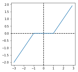
Donde $S_\theta(x)$ es la función soft-threshold definida como

$S_\theta(x) = \left\{\begin{matrix} x-\theta & x >\theta \\ 0 & -\theta \le x \le \theta \\ x+\theta & x< \theta \end{matrix} \right.$

import matplotlib.pyplot as plt
import numpy as np

#-------------------------------------
# Soft Treshold function
def softTreshold (x, theshold=1):
    s = np.zeros(x.shape)
    idx = x < -theshold
    s[idx] = x[idx]+theshold
    idx = x >  theshold
    s[idx] = x[idx]-theshold
    return s
#-------------------------------------

x = np.arange(-3.0, 3.0, 0.1)
plt.figure(figsize=(4,4))
plt.axvline(0.0, ls='dashed', color='k')
plt.axhline(0.0, ls='dashed', color='k')
plt.plot(x,softTreshold(x, theshold=1))
plt.show()

Ejemplo de Regresión LASSO

import numpy as np
import scipy.linalg as spla

m=1000
n=2
theta = np.random.rand(3)
print(theta)

# Matriz de diseño real
x = np.random.rand(m,n)
X = np.concatenate((np.ones((m,1)),x), axis=1)
n = 0.1*np.random.randn(m)

# variable dependiente
y = X@theta + n

# Matriz de diseño extendida
Xn =  np.concatenate((X, x**2), axis=1) 

[ 0.01945935  0.57451632  0.28247946]

Solución mediante AMDD

1. $x = (A^\top A+ \rho I )^{-1} A^\top b + \rho z - u$

2. $z = S_{\frac{\lambda}{\rho}}(x + u/\rho)$

3. $u = u + \rho \, (x-z)$

#-------------------------------------
def ls_AMDD_LASSO(X, y, Lambda=.1, rho=.1, niter = 10, epsilon = 1e-2):
    (m,n) = X.shape
    theta = np.zeros(n)
    u = np.zeros(n)
    z = np.zeros(n)
    M = spla.inv(X.T@X + rho*np.eye(n)) @ X.T
    for t in range(niter):
        theta =  M@y + rho*z - u
        z = softTreshold (theta+u/rho, theshold=Lambda/rho)
        delta=theta-z
        if spla.norm(delta) < epsilon:
            break
        u += rho*delta
        
    return (theta, z, u, delta, t)
#-------------------------------------

thetaLasso, z, u, delta, t = ls_AMDD_LASSO(Xn, y, Lambda=.05, rho=.1, niter=1000, epsilon =1e-5)
print(z,t)
print(thetaLasso)

[ 0.          0.54280946  0.19837477  0.          0.        ] 85
[  4.60236042e-06   5.42809456e-01   1.98374767e-01   5.41948371e-06
   6.35802127e-06]