FEMT is an open source muli-platform library and tools (Windows, Linux and Mac OS) for solving large sparse systems of equations in parallel. This software is specialy set to solve systems of equations resulting from finite element, finite volume and finite differences discretizations.
The library and tools are in continuos development, but they are quite stable, currently our research group use them in several other projects.
The FEMT source code is basically divided in three parts:
Paper.FEMT.pdf (preprint).
FEMT.Manual.2012Nov29.pdf (It is a very first draft).
https://www.microsoft.com/en-us/download/confirmation.aspx?id=48145October 7, 2015. FEMT-beta36.tar.xz (478,564 bytes).
• Windows binaries: tools-beta36-win32.zip (246,567 bytes), gid-problemtypes-beta36-win32.zip (526,701 bytes), you may need Visual C++ Redistributable to run them.
September 22, 2015. FEMT-beta35.tar.xz (473,480 bytes)
September 18, 2015. FEMT-beta34.tar.xz (471,864 bytes)
November 29th, 2012. FEMT-beta33.tar.bz2 (698,882 bytes)
October 28th, 2012. FEMT-beta32.tar.bz2 (698,421 bytes)
June 20th, 2012. FEMT-beta31.tar.bz2 (670,200 bytes)
May 29th, 2012. FEMT-beta30.tar.bz2 (672,851 bytes) tools-win32.zip (290,043 bytes) tools-win64.zip (387,299 bytes)
May 27th, 2012. FEMT-beta29.tar.bz2 (672,670 bytes)
May 10th, 2012. FEMT-beta28.tar.bz2 (682,442 bytes)
April 18th, 2012. FEMT-beta27.tar.bz2 (668,377 bytes)
March 21st, 2012. FEMT-beta23.tar.bz2 (673,577 bytes)
Note: for using the windows binaries you will need to have installed the Microsoft Visual C++ 2008 Redistributable Package (32 bits or 64 bits). If you want to use the MPI solvers you will also need to install the MPICH2 library (32 bits or 64 bits).
By default only solvers implemented with OpenMP will be build, but if you have installed an MPI library you can also build the MPI solver.
A recent version of GCC (>= 4.3) is needed, you can also use the Intel C++ compiler (>= 10.1).
Optionally you can use MPI, I have tested with Open-MPI and MPICH2 (if the library is installed it will be detected in the Makefile).
tar xjf FEMT-<version>.tar.bz2
cd FEMT-<version>
make -C build/gcc
Currently only Visual Studio Community 2015 is supported, support for building FEMT with GCC for Windows (MinGW) is on testing stage.
For MPI, I only have tested MPICH2 for Windows (32 bits or 64 bits). Once you have installed MPICH2, you have to make it available for Visual Studio, to do so, run Visual Studio and click on the menu "Tools/Options", on the dialog select "Projects and Solutions/VC++ Directories". Now select to "Show directories for:" "Include files", there add a new item to point to the include directory of your MPICH2 installation (for example "C:\Program Files\MPICH2-ia32\include"). After that select "Show directories for:" "Library files" and add an item for the lib directory (for example "C:\Program Files\MPICH2\lib").
The solution file for Visual Studio is located in "build\VisualC++\All.sln".
There are four build configurations defined:
You have to select the "no MPI" configurations if you don't have/want to use the MPI solver.
To select the configuration click on the menu "Build/Configuration Manager", you can also select the platform: Win32 or x64.
Press F7 to build the solution.
This tutorial will explain briefly how to use the tools included in FEMT. Instructions are similar for all platforms. Commands for GNU/Linux and Mac OS will be to the left and commands for Windows will be to the right.
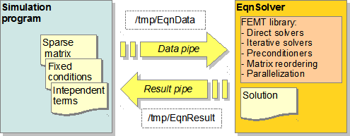
This program was designed to solve sparse systems of equations from finite element, finite volume and finite differences problems in parallel using the FEMT library on multi-core computers. Data is send to EqnSolver using named pipes. A named pipe is an object of the operationg system that can be accessed like a file but does not write data to the disk, is a fast way to communicate two running programs. One program will be your simulation program the other will be the EqnSolver.
If you know how make programs to read and write files, you can use EqnSolver. The user only needs to write on a named pipe the sparse systeme of equations (using compress row storage), the fixed conditions, and the vector of intependent terms. EqnSolver reads these data and runs one of the solvers from the FEMT library and retuns the solution using other named pipe, the user only has to read it like reading a normal file.
By default the named pipe used to send commands to EqnSolver is named "EqnData", on Linux and Mac OS systems it is located in "/tmp/EqnData", on Window its name is "\\.\pipe\EqnData". The results pipe is named "EqnResult"
First open a console, go to the "tools" directory and run "EqnSolver":
| on GNU/Linux and Mac OS: | on Windows: | |
|---|---|---|
cd FEMT-beta30/tools ./EqnSolver [ 0.000] EqnSolver ----------------------------- [ 0.001] Version: beta30 [ 0.002] Solver -------------------------------- [ 0.002] -Type: Conjugate gradient [ 0.003] -Threads: 1 [ 0.003] -Reorder equations: no [ 0.004] -Tolerance: 1e-05 [ 0.006] -Maximum steps: 10000 [ 0.006] -Preconditioner: Jacobi [ 0.007] -Level: 1 [ 0.007] Create pipes -------------------------- [ 0.008] Data pipe: /tmp/EqnData [ 0.008] Result pipe: /tmp/EqnResult | cd FEMT-beta30\tools EqnSolver.exe [ 0.000] EqnSolver ----------------------------- [ 0.002] Version: beta30 [ 0.004] Solver -------------------------------- [ 0.007] -Type: Conjugate gradient [ 0.012] -Threads: 1 [ 0.016] -Reorder equations: no [ 0.021] -Tolerance: 1e-005 [ 0.026] -Maximum steps: 10000 [ 0.031] -Preconditioner: Jacobi [ 0.036] -Level: 1 [ 0.041] Create pipes -------------------------- [ 0.045] Data pipe: \\.\pipe\EqnData [ 0.050] Result pipe: \\.\pipe\EqnResult |
When you run EqnSolver it display its configuration, creates the two pipes and then stops running until something is written to the data pipe. The numbers on the left are the elapsed time
In the same "tools" directory there is a small example to test EqnSolver, this example solves a heat difussion problem with 22 degrees of freedom. To run it, open other console, go to the same directory and execute:
| on GNU/Linux and Mac OS: | on Windows: | |
|---|---|---|
cd FEMT-beta30/tools ./EqnSolverExample_cpp 273.000000 273.000000 268.766629 270.716406 271.597080 267.665508 273.000000 262.985334 271.423243 261.967666 270.925926 270.522499 270.229477 272.755261 277.245797 265.725972 268.280490 275.513072 268.338864 277.096765 293.000000 270.876208 | cd FEMT-beta30\tools EqnSolverExample.exe 273.000000 273.000000 268.766629 270.716406 271.597080 267.665508 273.000000 262.985334 271.423243 261.967666 270.925926 270.522499 270.229477 272.755261 277.245797 265.725972 268.280490 275.513072 268.338864 277.096765 293.000000 270.876208 |
The numbers shown are the temperature in each node of the mesh.
You will see that on the console that is running EqnSolver some information is displayed at the same time:
| on GNU/Linux and Mac OS: | on Windows: | |
|---|---|---|
[ 5.662] ConjugateGradientJacobi: [ 5.663] -Tolerance: 1.00000e-05 [ 5.664] -MaxSteps: 10000 [ 5.664] -Step r'*r [ 5.665] 0 7.33375e-04 [ 5.665] 1 6.12597e-04 [ 5.666] 2 4.27307e-04 [ 5.666] 3 6.33109e-05 [ 5.667] 4 1.72719e-05 [ 5.668] 5 7.18309e-07 [ 5.668] 6 2.42328e-08 [ 5.669] 7 8.31901e-09 [ 5.669] 8 3.26289e-09 [ 5.670] 9 7.39395e-10 [ 5.670] 10 2.18562e-11 [ 5.670] -Total steps: 11 [ 5.670] Solution: valid [ 5.679] Peak allocated memory: 4424 bytes | [ 6.552] ConjugateGradientJacobi: [ 6.555] -Tolerance: 1.00000e-005 [ 6.559] -MaxSteps: 10000 [ 6.562] -Step r'*r [ 6.565] 0 7.33375e-004 [ 6.568] 1 6.12597e-004 [ 6.572] 2 4.27307e-004 [ 6.575] 3 6.33109e-005 [ 6.579] 4 1.72719e-005 [ 6.582] 5 7.18309e-007 [ 6.585] 6 2.42328e-008 [ 6.588] 7 8.31901e-009 [ 6.593] 8 3.26289e-009 [ 6.596] 9 7.39395e-010 [ 6.600] 10 2.18562e-011 [ 6.603] -Total steps: 11 [ 6.606] Solution: valid [ 6.706] Peak allocated memory: 3743 bytes |
What happened here is that the EqnSolverExample program sended to EqnSolver the problem data through the data pipe, EqnSolver read the system of equations, ran the conjugate gradient with Jacobi precontidioner to solve the system, it took 10 steps to converge and returned a vector using the result pipe. The values shown in each step are the squared norm of the residual.
This example was made in C, but it the simulation program can be made in any languaje.
The directory "source/Examples/EqnSolverExample/" contains the examples, in Python, C and Fortran
Let's examine how the communication is done using the Python version:
import sys import array | These are the only imports needed |
command_end         = array.array('b', [0])
command_set_size    = array.array('b', [1])
command_set_row     = array.array('b', [2])
command_set_x       = array.array('b', [3])
command_set_b       = array.array('b', [4])
command_set_fixed   = array.array('b', [5])
command_solver_init = array.array('b', [6])
command_solver_run  = array.array('b', [7])
| These are the commands that can be send to EqnSolver |
M = 22 | Number of equations |
values = [ \
  array.array('d', [ 1.2326e-4, -3.6051e-5, -3.3996e-5, -5.3214e-5]), \
  array.array('d', [-3.6051e-5,  1.7051e-4, -4.3495e-5, -6.0877e-5, -3.0080e-5]), \
  array.array('d', [-3.3996e-5,  1.7031e-4, -5.5748e-5, -4.5665e-5, -3.4908e-5]), \
  array.array('d', [-5.3214e-5, -4.3495e-5, -5.5748e-5,  3.4166e-4, -7.1143e-5, -6.8663e-5, -4.9398e-5]), \
  array.array('d', [-6.0877e-5, -7.1143e-5,  3.4266e-4, -5.8603e-5, -4.4280e-5, -4.3101e-5, -6.4660e-5]), \
  array.array('d', [-4.5665e-5, -6.8663e-5,  3.4154e-4, -5.6229e-5, -4.4270e-5, -5.8971e-5, -6.7747e-5]), \
  array.array('d', [-3.0080e-5, -5.8603e-5,  1.2279e-4, -3.4101e-5]), \
  array.array('d', [-3.4908e-5, -5.6229e-5,  1.2291e-4, -3.1776e-5]), \
  array.array('d', [-4.9398e-5, -4.4280e-5, -4.4270e-5,  3.29610e-4, -4.7225e-5, -5.2776e-5, -5.2312e-5, -3.934e-5]), \
  array.array('d', [-5.8971e-5, -3.1776e-5,  1.7029e-4, -4.4634e-5, -3.4908e-5]), \
  array.array('d', [-4.3101e-5, -3.4101e-5,  1.7088e-4, -6.6464e-5, -2.7214e-5]), \
  array.array('d', [-6.4660e-5, -4.7225e-5, -6.6464e-5,  3.4233e-4, -5.0917e-5, -6.2790e-5, -5.0269e-5]), \
  array.array('d', [-6.7747e-5, -5.2776e-5, -4.4634e-5,  3.4104e-4, -5.8172e-5, -5.6229e-5, -6.1479e-5]), \
  array.array('d', [-5.2312e-5, -5.0917e-5,  3.4252e-4, -7.1496e-5, -5.5711e-5, -5.1107e-5, -6.0978e-5]), \
  array.array('d', [-3.9340e-5, -5.8172e-5, -7.1496e-5,  3.4468e-4, -4.5355e-5, -6.3923e-5, -6.6385e-5]), \
  array.array('d', [-3.4908e-5, -5.6229e-5,  1.2291e-4, -3.1776e-5]), \
  array.array('d', [-2.7214e-5, -6.2790e-5,  1.2287e-4, -3.2858e-5]), \
  array.array('d', [-6.1479e-5, -4.5355e-5, -3.1776e-5,  1.7057e-4, -3.1962e-5]), \
  array.array('d', [-5.0269e-5, -5.5711e-5, -3.2858e-5,  1.7088e-4, -3.2040e-5]), \
  array.array('d', [-5.1107e-5, -6.3923e-5,  1.6949e-4, -2.4862e-5, -2.9603e-5]), \
  array.array('d', [-6.6385e-5, -3.1962e-5, -2.4862e-5,  1.2321e-4]), \
  array.array('d', [-6.0978e-5, -3.2040e-5, -2.9603e-5,  1.2262e-4])]
| Sparse matrix values, non zero entries in each row |
indexes = [ \
  array.array('i', [1, 2, 3, 4]), \
  array.array('i', [1, 2, 4, 5, 7]), \
  array.array('i', [1, 3, 4, 6, 8]), \
  array.array('i', [1, 2, 3, 4, 5, 6, 9]), \
  array.array('i', [2, 4, 5, 7, 9, 11, 12]), \
  array.array('i', [3, 4, 6, 8, 9, 10, 13]), \
  array.array('i', [2, 5, 7, 11]), \
  array.array('i', [3, 6, 8, 10]), \
  array.array('i', [4, 5, 6, 9, 12, 13, 14, 15]), \
  array.array('i', [6, 8, 10, 13, 16]), \
  array.array('i', [5, 7, 11, 12, 17]), \
  array.array('i', [5, 9, 11, 12, 14, 17, 19]), \
  array.array('i', [6, 9, 10, 13, 15, 16, 18]), \
  array.array('i', [9, 12, 14, 15, 19, 20, 22]), \
  array.array('i', [9, 13, 14, 15, 18, 20, 21]), \
  array.array('i', [10, 13, 16, 18]), \
  array.array('i', [11, 12, 17, 19]), \
  array.array('i', [13, 15, 16, 18, 21]), \
  array.array('i', [12, 14, 17, 19, 22]), \
  array.array('i', [14, 15, 20, 21, 22]), \
  array.array('i', [15, 18, 20, 21]), \
  array.array('i', [14, 19, 20, 22])]
| Indexes of non zero entries in each row |
count = array.array('i', [4, 5, 5, 7, 7, 7, 4, 4, 8, 5, 5, 7, 7, 7, 7, 4, 4, 5, 5, 5, 4, 4])
| Number of non zero entries in each row |
x = array.array('d', [273, 273, 0, 0, 0, 0, 273, 0, 0, 0, 0, 0, 0, 0, 0, 0, 0, 0, 0, 0, 293, 0])
| Vector with constrain values |
b = array.array('d', [0, 0, 0, 0, 0, 0, 0, -4.3388e-4, 0, -8.6776e-4, 0, \
  0, 0, 0, 0, -4.3388e-4, -2.1694e-4, 0, -4.3388e-4, 0, 0, -2.1694e-4])
| Vector of independent terms |
fixed = array.array('b', [1, 1, 0, 0, 0, 0, 1, 0, 0, 0, 0, 0, 0, 0, 0, 0, 0, 0, 0, 0, 1, 0])
| Vector that indicates where the constrains are |
r = array.array('d')
| Result vector |
if sys.platform == "win32": dataname = r'\\.\pipe\EqnData' resultname = r'\\.\pipe\EqnResult' else: dataname = r'/tmp/EqnData' resultname = r'/tmp/EqnResult' | Paths for the pipes |
EqnData = open(dataname, "wb") EqnResult = open(resultname, "rb") | Open data and result pipes |
command_set_size.tofile(EqnData)
array.array('i', [M]).tofile(EqnData)
| Send number of equations |
for i in range(0, M):
  command_set_row.tofile(EqnData)
  array.array('i', [i + 1]).tofile(EqnData)
  array.array('i', [count[i]]).tofile(EqnData)
  indexes[i].tofile(EqnData)
  values[i].tofile(EqnData)
| For each row send: row number row size indexes values |
command_set_x.tofile(EqnData) x.tofile(EqnData) | Send vector with constrain values |
command_set_b.tofile(EqnData) b.tofile(EqnData) | Send vector of independent terms |
command_set_fixed.tofile(EqnData) fixed.tofile(EqnData) | Send vector that indicates where the constrains are |
command_solver_init.tofile(EqnData) | Initialize solver |
command_solver_run.tofile(EqnData) EqnData.flush() r.fromfile(EqnResult, M) | Run solver and read result |
for v in r[:]:
    print(v)
| Display result |
command_end.tofile(EqnData) | Send end session command |
EqnResult.close() EqnData.close() | Close pipes |
The communication with EqnSolver is done using commands, a command is a number (a single byte), most commands need some data after the command, for example, to indicate the number of equations you must write the value "1" (a single byte) to the pipe, then an integer (4 bytes) with the number of equations. Other example, the command "2" is used to send a row using compressed row storage, after the command the row number is send (integer, 4 bytes), then the size (integer, 4 bytes), and indexes (integers, 4 bytes for each one) and values (double precision float, 8 bytes for each one) of non zero entries.
The solver_init command needs to be sent after when all the system of equations is already sent, this command creates the preconditioner or factorization needed to solve the system. The solver_run command runs the solver routine.
Several parameters can be changed to set different solvers or number of threads, these parameters are set using environment variables.
For example, to use the Cholesky factorization with 4 threads we have to set SOLVER_TYPE=2 and SOLVER_THREADS=4 and then run aganin EqnSolver:
| on GNU/Linux and Mac OS: | on Windows: | |
|---|---|---|
export SOLVER_TYPE=2 export SOLVER_THREADS=4 ./EqnSolver [ 0.000] EqnSolver ----------------------------- [ 0.002] Version: beta30 [ 0.002] Solver -------------------------------- [ 0.003] -Type: Cholesky decomposition [ 0.003] -Threads: 4 [ 0.004] -Reorder equations: yes [ 0.005] Create pipes -------------------------- [ 0.005] Data pipe: /tmp/EqnData [ 0.006] Result pipe: /tmp/EqnResult | cd FEMT-beta30\tools EqnSolver.exe [ 0.000] EqnSolver ----------------------------- [ 0.003] Version: beta30 [ 0.004] Solver -------------------------------- [ 0.011] -Type: Cholesky decomposition [ 0.013] -Threads: 4 [ 0.017] -Reorder equations: yes [ 0.022] Create pipes -------------------------- [ 0.026] Data pipe: \\.\pipe\EqnData [ 0.031] Result pipe: \\.\pipe\EqnResult |
On the other console you can run the example again, it will be solved in parallel (if your computer is multi-core) using the Cholesky factorization.
For maximum performance you have to set the number of threads equal to the number of cores in your computer.
The full list of parameters that can be set are described in the file "tools\RunEqnSolver.cmd" for Windows and "tools/RunEqnSolver.sh" for GNU/Linux and Mac OS.
FEMSolver is a program that solves finite element problems in parallel using the FEMT library on multi-core computers. It is similar to EqnSolver, but instead of sending the system of equations you have to send the elemental matrices. Data is send to FEMSolver using named pipes. A named pipe is an object of the operationg system that can be accessed like a file but does not write data to the disk, is a fast way to communicate two running programs. One program will be your simulation program the other will be the FEMSolver.
The user only needs to write on a named pipe the connectivity matrix, the elemental matrices, the fixed conditions, and the vector of intependent terms. FEMSolver reads these data and runs one of the solvers from the FEMT library and retuns the solution using other named pipe, the user only has to read it like reading a normal file.
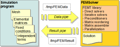
By default the named pipe used to send commands to FEMSolver is named "FEMData", on Linux and Mac OS systems it is located in "/tmp/FEMData", on Window its name is "\\.\pipe\FEMData". The results pipe is named "FEMResult"
First open a console, go to the "tools" directory and run "FEMSolver":
| on GNU/Linux and Mac OS: | on Windows: | |
|---|---|---|
cd FEMT-beta30/tools ./FEMSolver [ 0.000] FEMSolver ----------------------------- [ 0.000] -Version: beta30 [ 0.001] Solver -------------------------------- [ 0.001] -Type: Conjugate gradient [ 0.001] -Threads: 1 [ 0.001] -Reorder equations: no [ 0.001] -Tolerance: 1e-05 [ 0.001] -Maximum steps: 10000 [ 0.001] -Preconditioner: Jacobi [ 0.001] -Level: 1 [ 0.001] Create pipes -------------------------- [ 0.001] Data pipe: /tmp/FEMData [ 0.001] Result pipe: /tmp/FEMResult | cd FEMT-beta30\tools FEMSolver.exe [ 0.000] FEMSolver ----------------------------- [ 0.001] -Version: beta30 [ 0.001] Solver -------------------------------- [ 0.002] -Type: Conjugate gradient [ 0.002] -Threads: 1 [ 0.002] -Reorder equations: no [ 0.003] -Tolerance: 1e-5 [ 0.004] -Maximum steps: 10000 [ 0.004] -Preconditioner: Jacobi [ 0.004] -Level: 1 [ 0.005] Create pipes -------------------------- [ 0.005] Data pipe: \\.\pipe\FEMData [ 0.005] Result pipe: \\.\pipe\FEMResult |
When you run FEMSolver it display its configuration, creates the two pipes and then stops running until something is written to the data pipe. The numbers on the left are the elapsed time
In the same "tools" directory there is a small example to test FEMSolver, this example solves a heat difussion problem with 17 degrees of freedom. To run it, open other console, go to the same directory and execute:
| on GNU/Linux and Mac OS: | on Windows: | |
|---|---|---|
cd FEMT-beta30/tools ./FEMSolverExample_cpp 289.239730 288.673440 288.084259 286.030610 287.173591 284.633436 287.149394 289.278171 281.278447 286.016320 283.371570 288.671351 281.272196 273.000000 287.137672 273.000000 283.361920 | cd FEMT-beta30\tools FEMSolverExample.exe 289.239730 288.673440 288.084259 286.030610 287.173591 284.633436 287.149394 289.278171 281.278447 286.016320 283.371570 288.671351 281.272196 273.000000 287.137672 273.000000 283.361920 |
The numbers shown are the temperature in each node of the mesh.
You will see that on the console that is running FEMSolver some information is displayed at the same time:
| on GNU/Linux and Mac OS: | on Windows: | |
|---|---|---|
[ 6.288] ConjugateGradientJacobi: [ 6.289] -Tolerance: 1.00000e-05 [ 6.289] -MaxSteps: 10000 [ 6.290] -Step r'*r [ 6.290] 0 5.79295e-04 [ 6.291] 1 3.39039e-04 [ 6.291] 2 3.19477e-04 [ 6.292] 3 6.26639e-04 [ 6.292] 4 1.69528e-04 [ 6.293] 5 8.71483e-06 [ 6.293] 6 1.91377e-06 [ 6.294] 7 4.09892e-07 [ 6.294] 8 1.29952e-07 [ 6.295] 9 6.14577e-09 [ 6.295] 10 3.68466e-10 [ 6.295] 11 1.37917e-12 [ 6.295] -Total steps: 12 [ 6.295] Solution: valid [ 6.319] Peak allocated memory: 6536 bytes | [ 3.047] ConjugateGradientJacobi: [ 3.050] -Tolerance: 1.00000e-5 [ 3.053] -MaxSteps: 10000 [ 3.056] -Step r'*r [ 3.061] 0 5.79295e-4 [ 3.064] 1 3.39039e-4 [ 3.067] 2 3.19477e-4 [ 3.070] 3 6.26639e-4 [ 3.074] 4 1.69528e-4 [ 3.078] 5 8.71483e-6 [ 3.081] 6 1.91377e-6 [ 3.084] 7 4.09892e-7 [ 3.087] 8 1.29952e-7 [ 3.091] 9 6.14577e-9 [ 3.095] 10 3.68466e-010 [ 3.098] 11 1.37917e-012 [ 3.101] -Total steps: 12 [ 3.103] Solution: valid [ 3.180] Peak allocated memory: 6281 bytes |
What happened here is that the FEMSolverExample program sended to FEMSolver the problem data through the data pipe, FEMSolver read the data, assembled the system of equations then ran the conjugate gradient with Jacobi precontidioner to solve the system, it took 12 steps to converge and returned a vector using the result pipe. The values shown in each step are the squared norm of the residual.
The directory "source/Examples/FEMSolverExample/" contains the examples, in Python, C and Fortran
Let's see the example in C:
#include <stdio.h> | This is the only include needed |
int main()
{
| |
  enum Command {
    command_end              = 0,
    command_set_connectivity = 1,
    command_fill_A           = 2,
    command_set_Ae           = 3,
    command_set_all_Ae       = 4,
    command_set_x            = 5,
    command_set_b            = 6,
    command_set_fixed        = 7,
    command_solver_init      = 8,
    command_solver_run       = 9};
| These are the commands that can be send to FEMSolver |
int E = 21; | Number of elements |
int M = 17; | Number of nodes |
int T = 2; | Element type (2=Triangle, 3=Quadrilateral, 4=Tetrahedra, 5=Hexahedra) |
int N = 3; | Nodes per element |
int D = 1; | Degrees of freedom on each node |
  int connectivity[21*3] = {
     3,  8,  5,
     3,  5,  1,
     5,  8, 12,
     7,  2,  4,
     7,  4, 11,
     4,  2,  1,
    17, 16, 13,
    17, 13, 15,
    13, 16, 14,
    12, 15, 10,
    10, 15, 13,
    12, 10,  5,
    14, 11,  9,
     9, 11,  4,
    14,  9, 13,
    10, 13,  6,
     6, 13,  9,
    10,  6,  5,
     6,  9,  4,
     5,  6,  4,
     1,  5,  4};
| Connectivity matrix |
  double Ke[21][3*3] ={
    {6.4699e-5, -2.6213e-5, -3.8485e-5, -2.6213e-5, 6.4699e-5, -3.8485e-5, -3.8485e-5, -3.8485e-5, 7.6971e-5},
    {1.1941e-4, -6.4851e-5, -5.4564e-5, -6.4851e-5, 6.4518e-5,  3.3253e-7, -5.4564e-5,  3.3253e-7, 5.4232e-5},
    {6.4518e-5, -6.4851e-5,  3.3254e-7, -6.4851e-5, 1.1941e-4, -5.4564e-5,  3.3254e-7, -5.4564e-5, 5.4232e-5},
    {6.4699e-5, -2.6213e-5, -3.8485e-5, -2.6213e-5, 6.4699e-5, -3.8485e-5, -3.8485e-5, -3.8485e-5, 7.6971e-5},
    {1.1941e-4, -6.4851e-5, -5.4564e-5, -6.4851e-5, 6.4518e-5,  3.3254e-7, -5.4564e-5,  3.3254e-7, 5.4232e-5},
    {6.4518e-5, -6.4851e-5,  3.3253e-7, -6.4851e-5, 1.1941e-4, -5.4564e-5,  3.3253e-7, -5.4564e-5, 5.4232e-5},
    {6.4699e-5, -2.6213e-5, -3.8485e-5, -2.6213e-5, 6.4699e-5, -3.8485e-5, -3.8485e-5, -3.8485e-5, 7.6971e-5},
    {1.1941e-4, -6.4851e-5, -5.4564e-5, -6.4851e-5, 6.4518e-5,  3.3253e-7, -5.4564e-5,  3.3253e-7, 5.4232e-5},
    {6.4518e-5, -6.4851e-5,  3.3253e-7, -6.4851e-5, 1.1941e-4, -5.4564e-5,  3.3253e-7, -5.4564e-5, 5.4232e-5},
    {6.4699e-5, -2.6213e-5, -3.8485e-5, -2.6213e-5, 6.4699e-5, -3.8485e-5, -3.8485e-5, -3.8485e-5, 7.6971e-5},
    {1.1819e-4, -6.4851e-5, -5.3346e-5, -6.4851e-5, 6.5184e-5, -3.3253e-7, -5.3346e-5, -3.3253e-7, 5.3678e-5},
    {6.5184e-5, -6.4851e-5, -3.3253e-7, -6.4851e-5, 1.1819e-4, -5.3346e-5, -3.3253e-7, -5.3346e-5, 5.3678e-5},
    {6.4699e-5, -2.6213e-5, -3.8485e-5, -2.6213e-5, 6.4699e-5, -3.8485e-5, -3.8485e-5, -3.8485e-5, 7.6971e-5},
    {1.1819e-4, -6.4851e-5, -5.3346e-5, -6.4851e-5, 6.5184e-5, -3.3255e-7, -5.3346e-5, -3.3255e-7, 5.3678e-5},
    {6.5184e-5, -6.4851e-5, -3.3253e-7, -6.4851e-5, 1.1819e-4, -5.3346e-5, -3.3253e-7, -5.3346e-5, 5.3679e-5},
    {6.4434e-5, -2.5551e-5, -3.8882e-5, -2.5551e-5, 6.4434e-5, -3.8882e-5, -3.8882e-5, -3.8882e-5, 7.7765e-5},
    {7.6740e-5, -3.9583e-5, -3.7157e-5, -3.9583e-5, 6.6011e-5, -2.6427e-5, -3.7157e-5, -2.6427e-5, 6.3585e-5},
    {6.6010e-5, -3.9583e-5, -2.6427e-5, -3.9583e-5, 7.6740e-5, -3.7157e-5, -2.6427e-5, -3.7157e-5, 6.3585e-5},
    {7.4932e-5, -3.8450e-5, -3.6482e-5, -3.8450e-5, 6.6423e-5, -2.7973e-5, -3.6482e-5, -2.7973e-5, 6.4456e-5},
    {6.0475e-5, -6.7551e-5,  7.0758e-6, -6.7551e-5, 1.3331e-4, -6.5760e-5,  7.0758e-6, -6.5760e-5, 5.8684e-5},
    {7.1839e-5, -3.5919e-5, -3.5919e-5, -3.5919e-5, 6.6664e-5, -3.0744e-5, -3.5919e-5, -3.0744e-5, 6.6664e-5}};
| Elemental matrices |
double x[17] = {0, 0, 0, 0, 0, 0, 0, 0, 0, 0, 0, 0, 0, 273, 0, 273, 0};
| Vector with constrain values |
  double b[17] = {2.8173e-4, 2.8173e-4, 0, 0, 0, 0, 2.8173e-4, 2.8173e-4,
    0, 0, 2.8173e-4, 2.8173e-4, 0, 0, 2.8173e-4, 0, 2.8173e-4};
| Vector of independent terms |
bool fixed[17] = {0, 0, 0, 0, 0, 0, 0, 0, 0, 0, 0, 0, 0, 1, 0, 1, 0};
| Vector that indicates where the constrains are |
double r[17]; | Space for result vector |
char command; | Variable to indicate command to be sent to FEMSolver |
FILE* FEMData; | Data pipe |
FILE* FEMResult; | Result pipe |
int i; | Variable for indexes |
#ifdef WIN32 const char* dataname = "\\\\.\\pipe\\FEMData"; const char* resultname = "\\\\.\\pipe\\FEMResult"; #else const char* dataname = "/tmp/FEMData"; const char* resultname = "/tmp/FEMResult"; #endif | Names for the pipes |
FEMData = fopen(dataname, "wb"); FEMResult = fopen(resultname, "rb"); | Open data and result pipes |
command = command_set_connectivity; fwrite(&command, 1, 1, FEMData); fwrite(&M, sizeof(int), 1, FEMData); fwrite(&E, sizeof(int), 1, FEMData); fwrite(&T, sizeof(int), 1, FEMData); fwrite(&N, sizeof(int), 1, FEMData); fwrite(&D, sizeof(int), 1, FEMData); fwrite(connectivity, sizeof(int), E*N, FEMData); | Send connectivity data: M, number of nodes E, number of elements T, element type N, nodes per element D, degrees of freedom connectivity matrix |
  command = command_set_Ae;
  for (i = 0; i < E; ++i)
  {
    int e = i + 1;
    fwrite(&command, 1, 1, FEMData);
    fwrite(&e, sizeof(int), 1, FEMData);
    fwrite(Ke[i], sizeof(double), N*N, FEMData);
  }
| Send elemental matrices |
command = command_set_x; fwrite(&command, 1, 1, FEMData); fwrite(x, sizeof(double), M, FEMData); | Send vector with constrain values |
command = command_set_b; fwrite(&command, 1, 1, FEMData); fwrite(b, sizeof(double), M, FEMData); | Send vector of independent terms |
command = command_set_fixed; fwrite(&command, 1, 1, FEMData); fwrite(fixed, sizeof(bool), M, FEMData); | Send vector that indicates where the constrains are |
command = command_solver_init; fwrite(&command, 1, 1, FEMData); | Initialize solver |
command = command_solver_run; fwrite(&command, 1, 1, FEMData); fflush(FEMData); fread(r, sizeof(double), M, FEMResult); | Run solver and read result |
  for (i = 0; i < M; ++i)
  {
    printf("%f\n", r[i]);
  }
| Display result |
command = command_end; fwrite(&command, 1, 1, FEMData); fflush(FEMData); | Send end session command |
fclose(FEMResult); fclose(FEMData); | Close pipes |
return 0; } |
Several parameters can be changed to set different solvers or number of threads, these parameters are set using environment variables. The full list of parameters that can be set are described in the file "tools\FEMEqnSolver.cmd" for Windows and "tools/FEMEqnSolver.sh" for GNU/Linux and Mac OS.
FEMSolver.Schur is used the same way as FEMSolver, this program uses the Schur substructuring method to solve the system of equations. It was programmed to be used with MPI, this is a parallelization library commonly used in clusters of computers. The execution is done using the "mpiexec" command, it creates several instances (processes) of FEMSolver.Schur that can be run in a single multi-core computer or in several computers of a cluster.
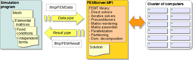
With this method the mesh is partitioned, the system of equations is splited into smaller systems that are solved in different computers.
From the user point of view it is used exactly as FEMSolver, it uses the same commands written to the same pipes. The difference is that FEMSolver.Schur has to be executed with the "mpiexec" command.
Open a console, go to the "tools" directory and run "FEMSolver.Schur" using the following command:
| on GNU/Linux and Mac OS: | on Windows: | |
|---|---|---|
cd FEMT-beta30/tools mpiexec -n 4 ./FEMSolver.Schur [ 0.000] FEMSolver.Schur ------------------------- [ 0.003] -Version: beta30 [ 0.003] -Partitions: 3 [ 0.003] Create pipes -------------------------- [ 0.003] Data pipe: /tmp/FEMData [ 0.003] Result pipe: /tmp/FEMResult | cd FEMT-beta30\tools "c:\Program Files\MPICH2\bin\mpiexec.exe" -n 4 FEMSolver.Schur.exe [ 0.000] FEMSolver.Schur ------------------------- [ 0.000] -Version: beta30 [ 0.000] -Partitions: 3 [ 0.000] Create pipes -------------------------- [ 0.000] Data pipe: \\.\pipe\FEMData [ 0.000] Result pipe: \\.\pipe\FEMResult |
The number after -n indicates the number of processes of FEMSolver.Schur to instanciate. FEMSolver.Schur uses one process to be the master process and n-1 to be the slave processes. Each slave process will handle a partition. So if you have to partition your mesh in 10 sub-domains, you have to use "mpiexec -n 11 FEMSolver.Schur".
Now, run the FEMSolverExample program again:
| on GNU/Linux and Mac OS: | on Windows: | |
|---|---|---|
cd FEMT-beta30/tools ./FEMSolverExample_cpp 289.239979 288.671738 288.085350 286.031747 287.173141 284.633374 287.148992 289.277489 281.279195 286.015827 283.370200 288.672412 281.271636 273.000000 287.137948 273.000000 283.362623 | cd FEMT-beta30\tools FEMSolverExample.exe 289.239979 288.671738 288.085350 286.031747 287.173141 284.633374 287.148992 289.277489 281.279195 286.015827 283.370200 288.672412 281.271636 273.000000 287.137948 273.000000 283.362623 |
The console that is running FEMSolver.Schur shows information about the solution:
| on GNU/Linux and Mac OS: | on Windows: | |
|---|---|---|
[ 6.135] Partitioning done [ 6.135] Systems of equations ------------------ [ 6.135] -Local solver threads: 4 [ 6.139] Partition 1: [ 6.139] Partition 2: [ 6.140] -Degrees of freedom: 9 (3 + 6) [ 6.140] -nnz(K): 39 [ 6.140] -Degrees of freedom: 8 (3 + 5) [ 6.140] -nnz(K): 36 [ 6.140] Partition 3: [ 6.140] -Degrees of freedom: 9 (3 + 6) [ 6.141] -nnz(K): 39 [ 6.142] Boundaries --------------------------- [ 6.143] -Degrees of freedom: 8 [ 6.143] -nnz(ABB): 30 [ 6.144] Substructuring ----------------------- [ 6.145] -Threads: 1 [ 6.146] -Tolerance: 1e-05 [ 6.170] -Step r'*r [ 6.171] 0 5.46672e-04 [ 6.172] 1 5.23740e-04 [ 6.173] 2 2.42611e-04 [ 6.174] 3 1.13649e-05 [ 6.174] 4 1.10283e-06 [ 6.176] 5 3.87584e-08 [ 6.177] 6 1.35271e-35 [ 6.177] -Total steps: 7 [ 6.179] Peak allocated memory ---------------- [ 6.179] -Master: 14664 bytes [ 6.179] -Partition 1: 2408 bytes [ 6.179] -Partition 2: 2440 bytes [ 6.179] -Partition 3: 2048 bytes [ 6.179] -Total: 21560 bytes | [ 2.392] Partitioning done [ 2.393] Systems of equations ----------------- [ 2.394] -Local solver threads: 1 [ 2.429] Partition 1: [ 2.429] -Degrees of freedom: 8 (3 + 5) [ 2.429] -nnz(K): 36 [ 2.429] Partition 2: [ 2.429] -Degrees of freedom: 9 (3 + 6) [ 2.429] -nnz(K): 39 [ 2.429] Partition 3: [ 2.430] -Degrees of freedom: 9 (3 + 6) [ 2.430] -nnz(K): 39 [ 2.431] Boundaries --------------------------- [ 2.431] -Degrees of freedom: 8 [ 2.431] -nnz(ABB): 30 [ 2.431] Substructuring ----------------------- [ 2.431] -Threads: 1 [ 2.431] -Tolerance: 1e-005 [ 2.438] -Step r'*r [ 2.439] 0 5.46672e-004 [ 2.439] 1 5.23740e-004 [ 2.439] 2 2.42611e-004 [ 2.439] 3 1.13649e-005 [ 2.439] 4 1.10283e-006 [ 2.439] 5 3.87584e-008 [ 2.439] 6 2.77231e-035 [ 2.439] -Total steps: 7 [ 2.439] Peak allocated memory ---------------- [ 2.439] -Master: 14589 bytes [ 2.439] -Partition 1: 1831 bytes [ 2.439] -Partition 2: 1902 bytes [ 2.439] -Partition 3: 1912 bytes [ 2.439] -Total: 20234 bytes |
Three environment variables contol FEMSolver.Schur, these are:
In order to pass these variables to FEMSolver.Shur you can create a script to set them, then you can run "mpiexec" to run this script. This is an example of a run script:
| run.sh | run.cmd | |
|---|---|---|
#!/bin/bash export SOLVER_THREADS=2 export SUBSTRUCTURING_THREADS=4 export SUBSTRUCTURING_TOLERANCE=1e-4 ./FEMSolver.Schur | @echo off set SOLVER_THREADS=2 set SUBSTRUCTURING_THREADS=4 set SUBSTRUCTURING_TOLERANCE=1e-4 FEMSolver.Schur.exe |
The command to run it would be:
| on GNU/Linux and Mac OS: | on Windows: | |
|---|---|---|
mpiexec -x LOG_LEVEL -n 4 ./run.sh | mpiexec -x LOG_LEVEL -n 4 run.cmd |
The parameters are described in the file "tools\FEMEqnSolver.Schur.cmd" for Windows and "tools/FEMEqnSolver.Schur.sh" for GNU/Linux and Mac OS.
Please, feel free to send questions and comments about FEMT to:
Jose Miguel Vargas-Felix 
Last modification: October 14th, 2015